How To Edit Pivot Table In Excel 2013
You can add and remove fields or instantly restructure the pivot table by dragging. If you change the size of your data set by adding or deleting rowscolumns you need to update the source data for the pivot table.
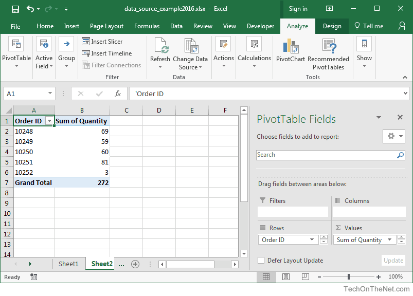
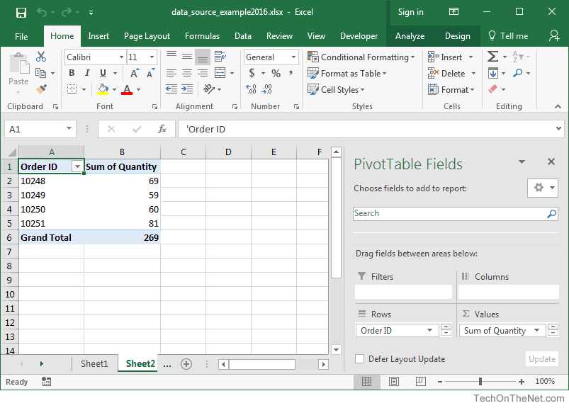
Ms Excel 2016 How To Change Data Source For A Pivot Table
Click anywhere in the PivotTable.

How to edit pivot table in excel 2013. Right click at any cell in the pivot table to show the context menu and select PivotTable Options. Edit a pivot table. Then on the Options tab of the PivotTable Tools ribbon click Fields Items Sets then choose Calculated Field.
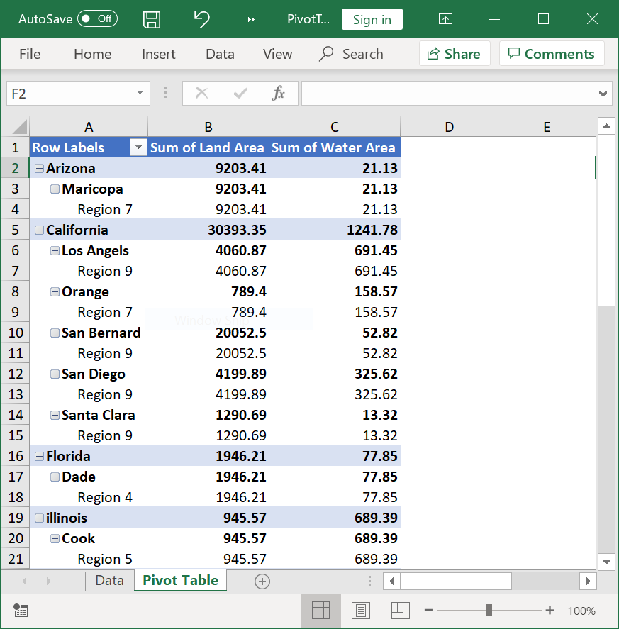
The steps below will walk through the process. First select any cell in the pivot table. And heres the resulting Pivot Table.
Somehow Excel is allowing me to edit values in the row labels of my Pivot table. The Enable cell editing in the values area is unchecked and in fact it is grayed out. Figure 2 Setting up the Data.
Is this a feature that has always been there and I just never noticed it. Now the pivot table is. Using that command with the Value option should do the job.
I do not care for it if it is a real feature. In the Data group click on Change Data Source button and select Change Data Source from the popup menu. In the PivotTable Options dialog box click the Layout Format tab and then under Layout select or clear the Merge and center cells with labels check box.
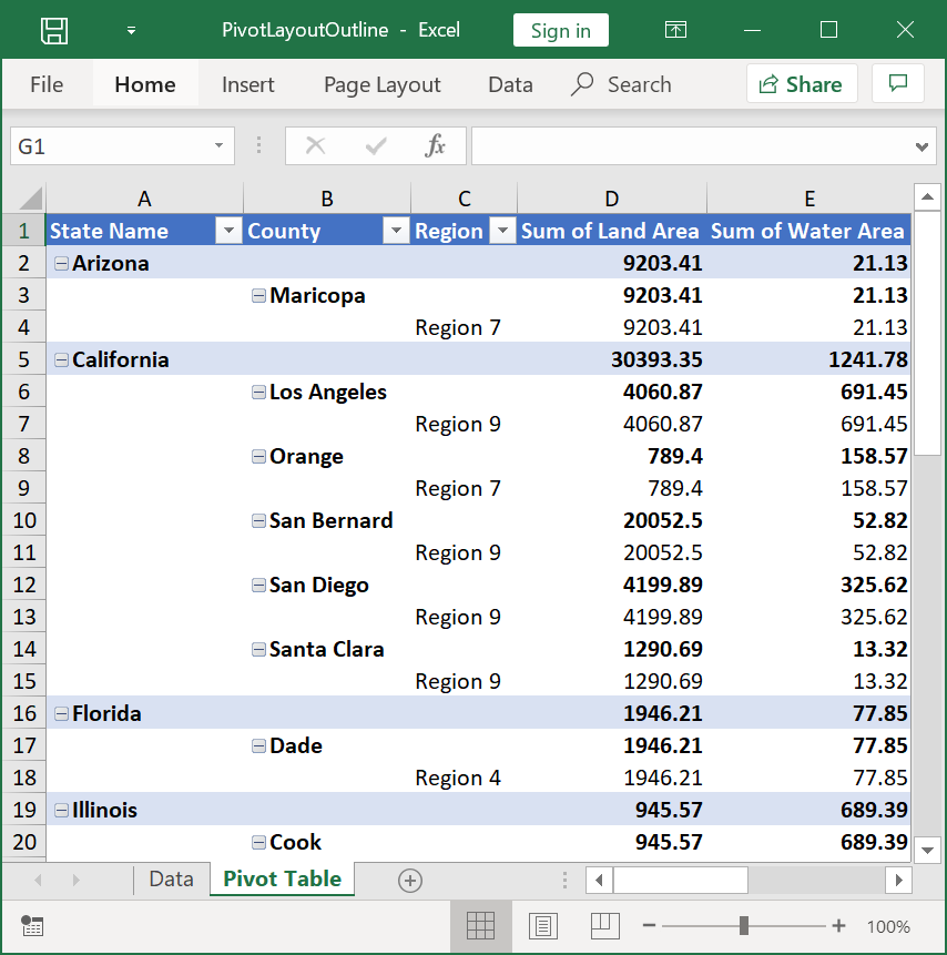
We can edit a PivotTable by removing or adding columns row or modify the data when there are new entries. Figure 1- How to Edit a Pivot Table in Excel. In the PivotTable Options dialog click Display tab and check Classic PivotTable Layout enables dragging fields in the grid option.
Excel doesnt have a command to unlink a pivot table but it does have a flexible Paste Special command. Display the Paste Special dialog box. Change your data set to a table before you insert a pivot table.
Add data Depending on where you want to add data under Rows Columns or Values click Add. Select the ANALYZE tab from the toolbar at the top of the screen. In this example weve chosen cells A1 to F16 in Sheet1.
How do I change the data source for an existing pivot table. We will click on one of the cells in the data rangeWe will go to the Insert tab and click on Pivot Table. Next choose the fields to add to the report.
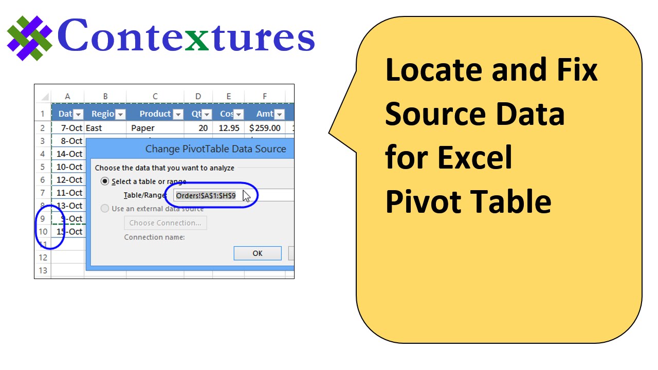
Change the Source Data for your Pivot Table. Next select the calculated field you want to. To use a different Excel table or cell range click Select a table or range and then enter the first cell in the Table.
Then in the pop-up dialog select the new data range you need to update. Click anywhere in a pivot table to open the editor. In the Tables group click on the Tables button and select PivotTable from the popup menu.
Do one of the following. Please follow the below steps to update pivot table range. To modify a calculated field you need to navigate to the Insert Calculated Field dialog box.
A Create PivotTable window should appear. Select the pivot table cells and press CtrlC to copy the range. This displays the PivotTable Tools tab on the ribbon.
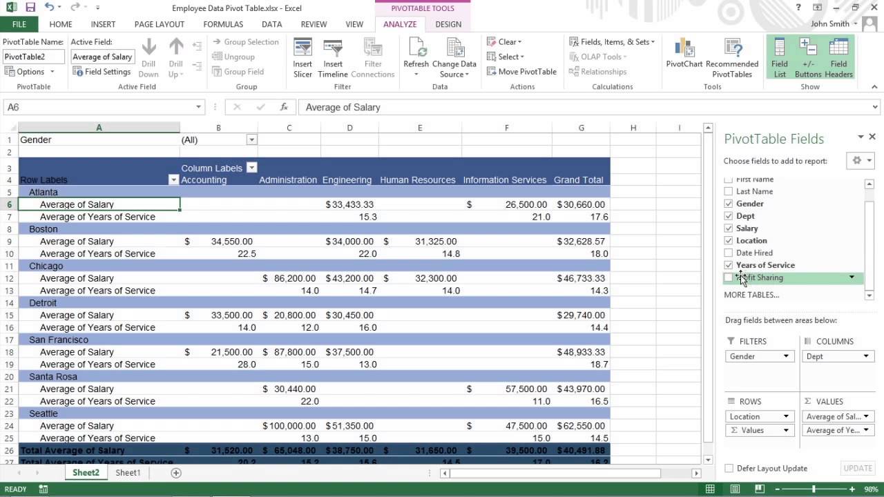
In Microsoft Excel 2013 Ive created a pivot table and now I need to change the data source. In order to change the source data for your Pivot Table you can follow these steps. On the Options tab in the Data group click Change Data Source and then click Change Data Source.
This way your. Click any cell inside the pivot table. Next we will confirm that the selected range is indeed the right rangeLast we will select New Worksheet to create.
Nov 09 2019 To create a new Pivot Table. On the Analyze tab in the Data group click Change Data Source. Click OK to close the dialog and now the pivot table layout change.
Select the range of data for the pivot table and click on the OK button. Add your new data to the existing data table. We will use the Pivot Table in figure 2 to illustrate how we can edit a Pivot Table.
Setting up the Data. Change row or column names Double-click a Row or Column name and enter a new name. In our case well simply paste the additional rows of data into the existing sales data table.
Right click on the cell Click on Value Field Setting Click on Number Format Apply the Required Formatting Click OK. The Change PivotTable Data source dialog box is displayed. Excel 2013 makes it easy to change the fields used in your pivot tables.
After you change the data range click the relative pivot table and click Option in Excel 2013 click ANALYZE Change Data Source. Change the formatting of the Pivot Table values. Pressing AltES is my favorite method and it works for all versions.
Change sort order or column Under Rows or Columns click the Down arrow under Order or. To change the formatting of values in the Pivot Table follow the steps below. On the Options tab in the PivotTable group click Options.
When the Change PivotTable Data Source window.
How To Move The Position Of A Pivot Table In An Excel Spreadsheet Quora
How To Find And Fix Excel Pivot Table Source Data

How To Count Unique Values In Pivot Table
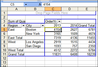
Format A Pivot Table In Excel 2003 Classic Style Excel Pivot Tables
Working With Pivot Tables Excel Library Syncfusion
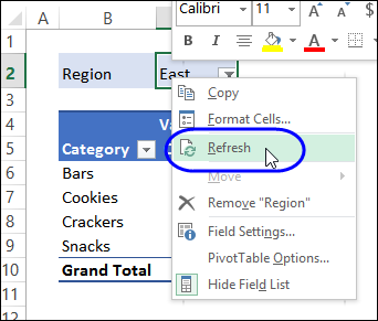
Automatically Refresh An Excel Pivot Table Excel Pivot Tables
Working With Pivot Tables Excel Library Syncfusion
Dynamic Pivot Table
How To Modify Pivot Tables In Excel 2013 For Dummies Youtube
Ms Excel 2013 How To Change Data Source For A Pivot Table
Ms Excel 2016 How To Change Data Source For A Pivot Table
Ms Excel 2010 How To Change Data Source For A Pivot Table
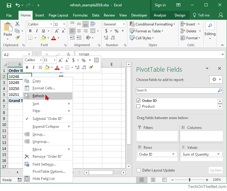
Ms Excel 2016 How To Refresh A Pivot Table
Excel Pivot Tables Add A Column With Custom Text Youtube

Applying Conditional Formatting To A Pivot Table In Excel

Working With Pivot Tables Excel Library Syncfusion

Pivot Table Excel The 2020 Tutorial Earn Excel
How To Delete A Pivot Table In Excel Easy Step By Step Guide
Ms Excel 2013 How To Create A Pivot Table
Posting Komentar untuk "How To Edit Pivot Table In Excel 2013"